Probability & Statistics

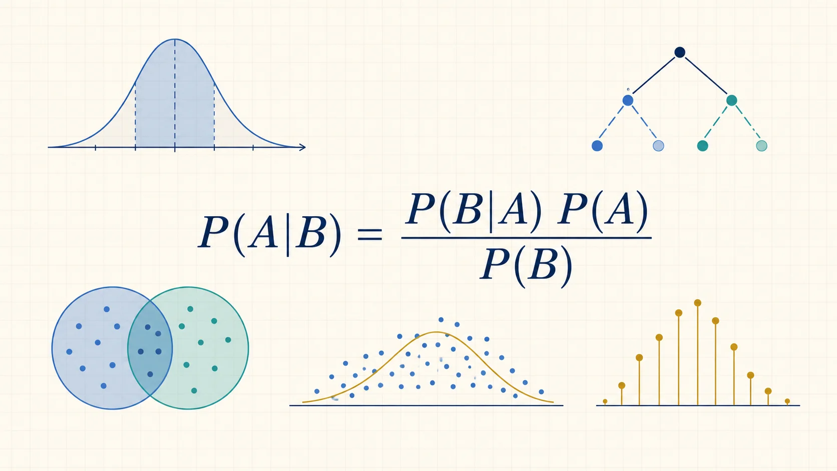
These are my personal reference notes on probability and statistics: a place to keep the definitions, derivations, and assumptions I find myself looking up. I’ve included explanations and examples so the equations make sense when I return to them later. Perhaps others will find them useful too.

Probability starts with a model and asks what data it could produce. Statistics works in the other direction: given some data, what can we learn about the process that produced it, and how uncertain should we be?

The notes move from probability and random variables to sample averages, inference, and regression. The formulas are useful as a reference, but their assumptions and interpretations are what make them usable.

Throughout, uppercase letters such as $X$ denote random variables, lowercase letters such as $x$ denote observed values, and a hat marks an estimate, such as $\hat{\theta}$. Expectations and variances are assumed to exist wherever they are used.

Probability

Events and the basic rules

A sample space $\Omega$ contains the possible outcomes of an experiment. An event $A$ is a set of those outcomes: for example, the event that a randomly selected component is defective. A probability assigns a number to each event according to three rules:

1. $P(A) \geq 0$ for every event $A$.
2. $P(\Omega) = 1$.
3. Probabilities add over a countable collection of disjoint events:

The third rule requires that the events cannot occur together. If events overlap, adding their probabilities counts the intersection twice. This gives the familiar inclusion–exclusion identity, alongside the complement and subset rules:

A frequentist interpretation connects probability to long-run frequencies in repeated experiments. A Bayesian interpretation also uses probability to express uncertainty given available information. Both use the same probability rules; their differences become more visible when we discuss unknown parameters.

Conditioning and independence

Conditioning restricts attention to outcomes compatible with some information. If $B$ has positive probability, then

Among the outcomes in $B$, this is the fraction that also belong to $A$. The conditioning event stays fixed while we apply the usual probability rules to events on the left of the bar. For disjoint $A_1$ and $A_2$, for example,

We cannot generally split a union on the right of the bar this way: changing what we condition on changes the population under consideration.

Two events are independent when knowing that one occurred does not change the probability of the other. Equivalently,

When $P(B)>0$, this implies $P(A \mid B)=P(A)$. Independence is different from mutual exclusivity. If two disjoint events both have positive probability, observing one rules out the other, so they cannot be independent. For more than two events, pairwise independence alone does not guarantee joint independence.

Total probability and Bayes’ rule

Suppose the events $A_i$ partition the sample space into nonoverlapping cases. We can find the probability of $B$ by averaging its conditional probability across those cases:

The same idea works within a conditioning event $C$:

where we only need conditional terms for cases with positive probability. Bayes’ rule reverses the direction of conditioning:

The denominator is often computed using total probability. This matters because $P(A \mid B)$ and $P(B \mid A)$ answer different questions.

For a concrete example, suppose 1% of components are defective. An inspection flags 90% of defective components, but also flags 5% of good ones. Writing $D$ for a defect and $F$ for a flag,

Only about 15.4% of flagged components are defective in this hypothetical population. Good components are so much more common that even a small false-positive rate contributes many flags. The prior prevalence, $P(D)$, is essential to interpreting the observation.

Random variables and distributions

From outcomes to numbers

A random variable is a function $X:\Omega \to \mathbb{R}$ that assigns a numerical value to an outcome. It might record the number of defective components in a batch, the waiting time until a machine fails, or a measurement error.

Its distribution describes how probability is allocated across possible values. The cumulative distribution function, or CDF, is

The CDF determines the distribution and works for both discrete and continuous variables. Two useful identities are

The endpoints matter when individual values have positive probability. If $X$ is an integer-valued count, for example, $P(X \geq 3)=1-F_X(2)$, not $1-F_X(3)$.

Probability mass and probability density

A discrete random variable has a probability mass function, or PMF:

For a variable with a probability density function, or PDF, probabilities instead come from areas:

The density is nonnegative, integrates to one, and satisfies $f_X(x)=F_X'(x)$ wherever the derivative exists. A density value is not itself a probability. For a uniform distribution on $[0,1/5]$, the density is 5 throughout the interval, but the total area is still one.

For a variable with a density, each individual point has probability zero. Including or excluding an interval endpoint therefore makes no difference to its probability. The PMF and PDF cases cover the distributions used below, although not every distribution has a density or is purely discrete.

Joint, marginal, and conditional distributions

A joint distribution describes several variables together. A marginal distribution removes variables we are not currently interested in by summing or integrating them out:

A conditional distribution keeps information about the other variable. Wherever $f_Y(y)>0$,

The analogous ratio holds for discrete probability masses. In the continuous case, this is a ratio of densities, even though the event $Y=y$ itself has probability zero.

Variables $X_1,\ldots,X_n$ are independent and identically distributed, or IID, when they are mutually independent and share the same distribution. Their joint mass or density then factors:

Identical distributions describe what the observations have in common; independence describes how they relate to one another. Repeated measurements can share a distribution while remaining correlated, so the two assumptions should be considered separately.

Transformations

To find the distribution of $Y=g(X)$, a reliable starting point is its CDF:

Rewrite the event in terms of $X$, then differentiate if $Y$ has a density. For example, if $X$ is uniform on $[0,1]$ and $Y=X^2$, then for $0<y<1$,

Squaring compresses values near zero, which explains why the transformed density is higher there.

Expectations and variation

Means and functions of random variables

An expectation is a probability-weighted average. For discrete and continuous variables, respectively,

It need not be a possible outcome: the expected value of a fair die is 3.5. Its usefulness is as a summary of the distribution and, under suitable conditions, the limit of repeated sample averages.

To compute the expectation of a transformed variable, we can work directly with the original distribution:

For a discrete variable, replace the integral with a sum. This is sometimes called the law of the unconscious statistician: there is no need to derive the distribution of $g(X)$ first.

Expectation is linear, whether or not the variables are independent:

Factoring expectations of products does require additional assumptions. For independent variables, $E[\prod_i X_i]=\prod_i E[X_i]$.

Variance, covariance, and correlation

Variance measures squared deviation from the mean:

The standard deviation is its square root, so it has the same units as $X$. Adding a constant changes the location but not the spread; multiplying by a constant rescales the spread:

Covariance measures how two variables vary together:

Correlation normalizes covariance by the standard deviations:

It lies between $-1$ and $1$ when both variances are positive. Independence implies zero covariance, but zero covariance does not generally imply independence: a nonlinear relationship can have no linear correlation.

Dependence also changes the variance of an aggregate:

For independent, or merely pairwise uncorrelated, variables, the covariance terms vanish. Positively correlated measurements provide less variance reduction from averaging than independent measurements do.

Conditional expectations and the total variance law

A conditional expectation averages within a specified value of another variable:

While $E[X]$ is a number, $E[X \mid Y]$ is a random variable: its value depends on the observed $Y$. Averaging those conditional means recovers the overall mean:

Similarly, conditional variance measures spread around the conditional mean:

The law of total variance separates overall variation into two sources:

If $Y$ identifies the machine that made a component and $X$ is its length, the first term measures average variation within machines. The second measures variation between the machines’ mean lengths. This distinction between unexplained variation and variation in conditional means will appear again in regression.

Common distributions

These distributions describe recurring kinds of uncertainty. Choosing among them means checking the process being modeled, not just matching the shape of a histogram.

Bernoulli: one binary outcome

A Bernoulli variable records success or failure, with possible values $x\in\{0,1\}$:

Here “success” is simply the outcome labeled 1; it might represent a defect. For $X\sim\operatorname{Bernoulli}(p)$,

The variance is largest at $p=1/2$, where the outcome is most uncertain, and zero at $p=0$ or $p=1$.

Binomial: successes in a fixed number of trials

The sum of $n$ independent Bernoulli variables with the same success probability is binomial. For $X\sim\operatorname{Binomial}(n,p)$ and $x=0,\ldots,n$,

The binomial coefficient counts the different trial sequences containing exactly $x$ successes. By adding the Bernoulli means and variances,

A fixed sample size, independent trials, and a common probability $p$ are all part of this model.

Geometric: waiting for the first success

If independent trials continue until a success occurs, let $X$ count the number of trials including the successful trial. For $0<p\leq 1$ and $x=1,2,\ldots$,

The first $x-1$ trials must fail and the last must succeed. For this convention,

Some references instead count failures before the success, giving support $0,1,\ldots$ and mean $(1-p)/p$. Checking the counting convention avoids an easy off-by-one error.

Normal: location and symmetric variation

The Normal, or Gaussian, distribution appears in measurement models and as an approximation to many sums and estimators. For $X\sim N(\mu,\sigma^2)$ with $\sigma>0$, its density is

The parameters are the mean $\mu$ and variance $\sigma^2$. Subtracting the mean and dividing by the standard deviation produces a standard Normal:

This lets us use one reference distribution for tail probabilities and quantiles. NIST’s Normal distribution reference collects these properties.

Sums of independent Normal variables are exactly Normal:

This exact result differs from the large-sample approximation supplied by the central limit theorem.

Multivariate Normal: correlated measurements

For a vector $\mathbf{X}$ with $k$ components, the multivariate Normal uses a mean vector $\boldsymbol{\mu}$ and covariance matrix $\Sigma$. When $\Sigma$ is positive definite, define

Then the density can be written as

The quadratic form $q$ measures squared distance from the mean after accounting for scale and correlation. The diagonal entries of $\Sigma$ are variances; the off-diagonal entries are covariances.

Within a jointly Normal vector, uncorrelated components are independent. That implication is special and does not hold for arbitrary joint distributions.

Chi-squared: sums of squared standardized quantities

If $Z_1,\ldots,Z_k$ are independent standard Normal variables, then

The parameter $k$ is the number of degrees of freedom. This distribution appears in variance estimation and in tests that combine squared discrepancies, such as Pearson’s test below.

Sample averages and convergence

Suppose $X_1,\ldots,X_n$ are IID with mean $\mu$ and finite variance $\sigma^2$. Their sample average is

Linearity gives $E[\bar{X}_n]=\mu$. Independence gives

The standard deviation of the average is therefore $\sigma/\sqrt{n}$. Quadrupling the number of independent observations halves this uncertainty. Correlated observations need a different calculation because their covariance terms do not disappear.

Law of large numbers: where the average goes

Under these assumptions, the sample average converges in probability to the population mean:

This means that, for any fixed tolerance $\epsilon>0$, the probability of an error larger than $\epsilon$ goes to zero. Chebyshev’s inequality gives a short proof:

Finite variance is sufficient for this proof. More general laws of large numbers can work under weaker conditions, but the conclusion here already explains why averages are useful estimates.

Central limit theorem: how the average fluctuates

The law of large numbers identifies the limit. The central limit theorem describes the shape of the remaining fluctuations. For IID observations with $0<\sigma^2<\infty$,

Equivalently, for sufficiently large $n$, we often approximate

The convergence statement applies to the standardized error; the second expression is a finite-sample approximation. The original observations need not be Normal. However, “sufficiently large” depends on their distribution, and strong skewness or heavy tails can make the approximation poor at sample sizes that work well elsewhere.

Statistical inference

Inference turns observations into estimates, intervals, and tests. In frequentist inference, the parameter is fixed and the procedure is evaluated over repeated random samples. Bayesian inference places a probability distribution on the parameter and updates it after conditioning on observed data. Both begin with a model for how observations arise.

Point estimates and sampling distributions

An estimator is a function of the sample:

Before we observe the data, it is a random variable. Afterward, it produces a numerical estimate. Its sampling distribution describes the values it would take across repeated samples from the same population.

Three quantities summarize different aspects of its behavior:

Bias measures systematic displacement from the target. Standard error measures variation across samples, rather than variation among individual observations. Mean squared error accounts for both:

An unbiased estimator can still be noisy, and a small amount of bias can sometimes buy a large reduction in variance. For a sample mean, the standard error is $\sigma/\sqrt{n}$; when $\sigma$ is unknown, we commonly estimate it with $s/\sqrt{n}$ using the sample standard deviation $s$.

Confidence intervals

A confidence interval is a data-dependent interval $C_n$ designed to contain a fixed parameter at a specified rate across repeated samples. An exact or conservative $1-\alpha$ procedure satisfies the following for every $\theta\in\Theta$:

The interval is random because its endpoints depend on the sample. Once the data are observed, the frequentist statement is about the procedure’s coverage, rather than a posterior probability assigned to the fixed parameter.

If an estimator’s standardized error is approximately standard Normal and its estimated standard error is reliable, an approximate interval is

where $z_q$ is the $q$ quantile of $N(0,1)$. For 95% confidence, $z_{0.975}\approx 1.96$. This approximation needs justification for the estimator at hand; it does not follow merely because some variable in the problem is Normal.

When an analytic sampling distribution is difficult to obtain, a bootstrap can approximate it by resampling the data. For IID observations, this usually means sampling observations with replacement and recomputing the estimate. Dependent data require a resampling scheme that preserves the relevant dependence.

Hypothesis tests and p-values

A hypothesis test compares a null model with an alternative:

We choose a statistic $T$ that captures a discrepancy from the null and reject for outcomes in a rejection region $R$. The probability of rejection depends on the true parameter:

For parameter values in the alternative, this is the test’s power. The size is the largest rejection probability within the null, $\sup_{\theta\in\Theta_0}\beta(\theta)$. A level-$\alpha$ test keeps that probability at most $\alpha$.

For a fully specified null distribution, a p-value is the probability of a statistic at least as extreme as the observed value, with “extreme” defined by the test. Composite nulls require an appropriate treatment of their unknown parameters. A p-value is not the probability that the null hypothesis is true, nor does it measure the size or practical importance of an effect.

Wald test

The Wald test asks how far an estimate lies from a null value, measured in standard errors. For $H_0:\theta=\theta_0$ against a two-sided alternative, use

If $W$ is approximately $N(0,1)$ under the null, reject when $|W|>z_{1-\alpha/2}$. The absolute value includes departures in both directions. This is equivalent to checking whether $\theta_0$ falls outside the matching Normal-approximation confidence interval.

Pearson’s chi-squared test

For categorical data, Pearson’s statistic compares observed counts $O_j$ with counts expected under the null, $E_j=np_{0j}$:

Suppose we roll a die $n$ times and test whether all six faces are equally likely. Each expected count is $n/6$, and large values of $T$ indicate a poor fit.

For multinomial observations with fixed, positive null probabilities and sufficiently large expected counts, the reference distribution is approximately $\chi^2_{K-1}$. One degree of freedom is lost because the counts sum to $n$. If $r$ identifiable parameters are fitted under the null by maximum likelihood, the usual regular-model adjustment is $K-1-r$. Sparse counts can make the chi-squared approximation unreliable.

Permutation tests

A permutation test constructs a reference distribution by rearranging the data in ways that would be equally plausible under the null. For two groups whose observations are exchangeable under the null, we can shuffle group labels and recompute a statistic such as the difference in means.

For a two-sided test, compare absolute differences. If $B$ random permutations produce statistics $T_1,\ldots,T_B$, a common Monte Carlo p-value is

The added observation prevents a p-value of zero simply because no sampled permutation was more extreme. The essential assumption is exchangeability under the null: arbitrary shuffling is invalid for data whose pairing, time dependence, or group structure must be preserved.

Parametric estimation

A parametric model restricts the possible data-generating distributions to a family indexed by $\theta$. This makes estimation more manageable, while making the conclusions depend on how well that family describes the data.

Maximum likelihood

For IID observations $x_1,\ldots,x_n$ from a mass or density $f(x\mid\theta)$, the likelihood is

The observed data stay fixed while we vary $\theta$. A likelihood therefore does not need to integrate to one over parameter values. The maximum likelihood estimate chooses the parameter that makes the observations most compatible with the model:

For Bernoulli observations with $s$ successes in $n$ trials, the log-likelihood is

Maximizing it gives $\hat{p}=s/n$, including the boundary estimates when all trials have the same outcome. The observed success rate is thus both an intuitive estimate and the MLE under this model.

Under identifiability and suitable regularity conditions, MLEs are consistent, asymptotically Normal, and asymptotically efficient among regular estimators. These are large-sample properties, not a guarantee of unbiasedness or low error in a small sample. Smoothness alone is insufficient.

MLEs are also invariant under one-to-one reparameterization: if $\hat{\theta}$ maximizes the likelihood for $\theta$, then $g(\hat{\theta})$ is the MLE for $g(\theta)$.

Likelihood ratio tests

Likelihood also provides a way to compare a restricted null model with a larger model containing it. Let $\hat{\theta}_0$ maximize the likelihood under the null restrictions and $\hat{\theta}$ maximize it in the full model. The statistic is

The full model can fit at least as well as the restricted model, so $\lambda$ is nonnegative. A large improvement in fit is evidence against the restrictions.

Under standard regularity conditions, $\lambda$ is asymptotically chi-squared under the null, with degrees of freedom equal to the difference in the models’ parameter dimensions. Boundary parameters and nonidentifiable models can invalidate this reference distribution. Unlike a Wald test, which starts with a parameter estimate and its standard error, this test directly compares optimized likelihoods.

Expectation maximization

Expectation maximization, or EM, is useful when a model includes unobserved variables $Z$, such as the unknown component assignments in a mixture model. If those variables were observed, fitting the complete-data model might be straightforward.

Starting from parameters $\theta^{(0)}$, repeat:

1. E-step: compute the expected complete-data log-likelihood using the current conditional distribution of $Z$:

2. M-step: choose parameters that maximize that expectation:

The expectation is over the log-likelihood, not simply over the missing values. Replacing every latent variable with its mean is generally a different procedure. In a mixture model, EM instead uses probabilistic component assignments.

With exact E- and M-steps, the observed-data likelihood does not decrease. This does not guarantee a global maximum; initialization can affect the result. Stanford’s EM notes derive the objective and explain this distinction.

Bayesian inference

Bayesian inference combines a likelihood with a prior distribution:

The prior represents uncertainty before observing $D$, the likelihood describes the data conditional on $\theta$, and the posterior represents uncertainty after conditioning on $D$. The denominator normalizes the posterior by averaging the likelihood over the prior.

For Bernoulli data, a Beta prior gives a simple example. If $p\sim\operatorname{Beta}(a,b)$ and the data contain $s$ successes in $n$ trials, then

The posterior mean is $(a+s)/(a+b+n)$. It combines prior information with the observed success rate, with the data receiving more weight as the sample grows.

A Bayesian credible interval contains a specified amount of posterior probability. Its interpretation is conditional on the observed data, prior, and model; this differs from the repeated-sample coverage interpretation of a confidence interval.

Linear regression

Regression brings these ideas together. We want to describe how an outcome varies with predictors, estimate that relationship from data, and quantify uncertainty in coefficients and predictions.

The conditional mean and the linear model

For a predictor vector $\mathbf{x}$, the regression function is

It describes the average outcome at those predictor values. Linear regression models this conditional mean as $\mathbf{x}^T\beta$. “Linear” refers to the coefficients: features may include transformations such as $x^2$, provided the model remains linear in $\beta$.

Let $X$ be an $n\times p$ design matrix whose $i$th row is $\mathbf{x}_i^T$, and let $Y$ be the vector of $n$ responses. Then

Here $p$ counts all coefficients, including an intercept if a column of ones is included. We assume $X$ has full column rank and $n>p$. The usual model for coefficient uncertainty is

The first condition makes $X\beta$ the conditional mean. The second says the errors have common variance and are uncorrelated across observations. With the stronger assumption of conditionally Gaussian errors,

We can compute least-squares point estimates without estimating $\sigma^2$. The noise variance becomes necessary for the standard errors and intervals below.

Least squares: algebra and geometry

Ordinary least squares minimizes the sum of squared residuals:

With independent Gaussian errors of common variance, this is also the MLE for $\beta$. Write the objective as $S(\beta)=\|Y-X\beta\|^2$. Expanding it gives

Because $X^TX$ is symmetric, the gradient simplifies to

Setting this to zero yields the normal equations and, when $X^TX$ is invertible, their solution:

Geometrically, $X\hat{\beta}$ is the projection of $Y$ onto the column space of $X$. At the closest point in that space, the residual is orthogonal to every column:

This is the same set of normal equations. The inverse formula is useful for derivations; numerical implementations generally solve the least-squares system using a factorization rather than explicitly forming the inverse.

Estimating noise and coefficient uncertainty

Write the residual vector as $\hat{\epsilon}=Y-X\hat{\beta}$. An unbiased estimate of the common error variance under the stated model is

The denominator accounts for the $p$ fitted coefficients. This measures spread around the fitted conditional mean, which is different from the overall spread of the observed responses.

Substituting the model into the coefficient estimator gives

Conditional on $X$, the randomness comes from $\epsilon$. Using its covariance yields

Replacing $\sigma^2$ by $\hat{\sigma}^2$ estimates this covariance matrix. For a compact notation, let $A=(X^TX)^{-1}$. The standard error of coefficient $j$ is the square root of the corresponding diagonal entry:

Under conditionally Gaussian errors, the standardized coefficient error has an exact Student’s $t$ distribution with $n-p$ degrees of freedom:

Writing $t_{\nu,q}$ for the $q$ quantile of that distribution, a $1-\alpha$ confidence interval is

To test $H_0:\beta_j=0$ against a two-sided alternative, reject when the absolute standardized coefficient exceeds the same critical value. Normal critical values provide a large-sample approximation when appropriate.

Estimating a mean versus predicting an observation

At new predictor values $\mathbf{x}_*$, the fitted conditional mean is

There are two different uncertainty questions. How accurately have we estimated the average response at $\mathbf{x}_*$? How far might one new response fall from that estimate?

Let $h_*=\mathbf{x}_*^T A\mathbf{x}_*$, with $A=(X^TX)^{-1}$ as above. The estimated standard error of the fitted mean is

A new observation also has its own error, independent of the training errors under the prediction model. The estimated standard deviation of its prediction error is therefore

The extra 1 represents the irreducible variation of that new observation. Even if the conditional mean were known exactly, individual responses would still vary around it.

Under the Gaussian model, a confidence interval for the mean response is

The wider prediction interval for one new response is

For example, estimating the average delivery time for a route is more precise than predicting the time of one particular delivery. Penn State’s regression lesson develops this distinction between confidence intervals for a mean and prediction intervals for an observation.

Which assumptions support which conclusions?

The formulas rely on different parts of the model. Keeping those dependencies separate makes it easier to understand what changes when an assumption fails.

• A conditional mean linear in the coefficients and zero conditional mean errors justify interpreting $X\beta$ as the mean response and make the full-rank OLS coefficient estimator conditionally unbiased.
• Full column rank makes the coefficients uniquely identifiable from this design. A feature that is an exact linear combination of others prevents the inverse formula from applying.
• Constant error variance and uncorrelated errors give the covariance and standard-error formulas above. Unequal variances or dependence require a different uncertainty calculation.
• Conditionally Gaussian errors give the exact finite-sample $t$ intervals and tests. Gaussian errors are not necessary to compute OLS estimates.
• A new observation following the same model, with an independent error, supports the prediction interval. Extrapolation can fail if the relationship changes outside the observed predictor range.

When using a statistical result, I find it helpful to identify the target first: an individual outcome, a population mean, a coefficient, or a whole distribution. Then I check which quantities are random, which assumptions justify the calculation, and what kind of uncertainty the result actually measures.