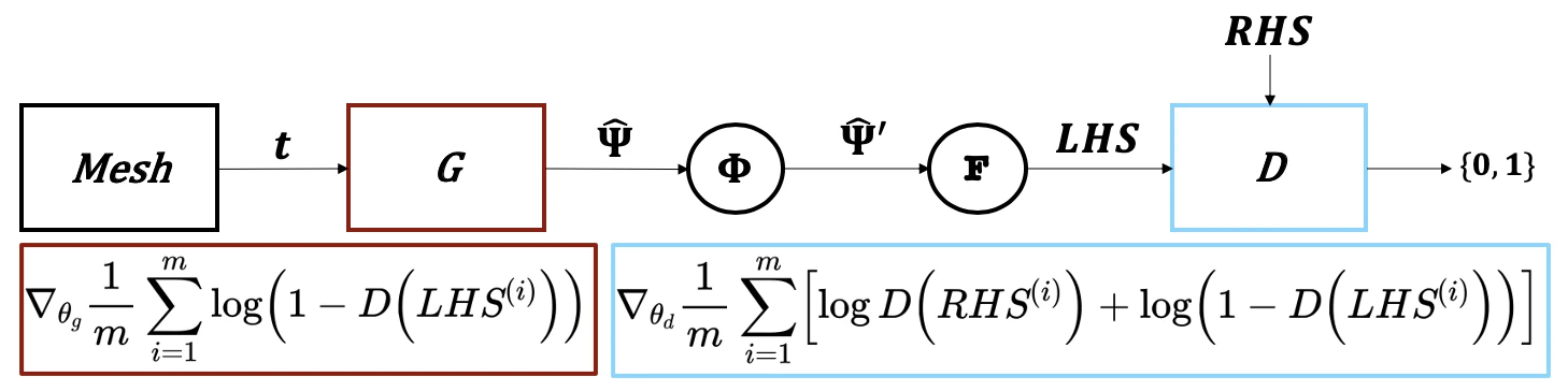
Physics-informed neural networks can solve differential equations without labeled examples: a network proposes a solution, automatic differentiation evaluates its derivatives, and training minimizes the equation’s residual. The usual approach still requires choosing a fixed residual loss such as L1, L2, or Huber loss.
In work presented at the AI4Science workshop at ICML 2022, we introduced Differential Equation GAN (DEQGAN). Instead of committing to one fixed residual penalty, DEQGAN trains a discriminator to learn the loss function used to improve the candidate solution.
Learning the residual loss
The generator maps sampled points in the problem domain to a candidate solution. We analytically reparameterize that output so it satisfies the prescribed initial or boundary conditions exactly, then use automatic differentiation to evaluate the governing equation.
For an equation written as
the discriminator receives the generator’s residuals as generated examples and zeros as real examples. Its job is to distinguish an imperfect solution from one that satisfies the equation; the generator learns to produce a solution whose residuals the discriminator cannot distinguish from zero. This adversarial game replaces a hand-selected residual norm with an adaptive objective.
We also studied several techniques for stabilizing training. Sampling a slightly different grid at every step reduced interpolation error, while residual connections, spectral normalization, and separate generator and discriminator learning rates improved optimization. Residual monitoring and adaptive instance noise made the method substantially more reliable across random initializations.
Evaluation
We evaluated DEQGAN on twelve ordinary and partial differential equations, ranging from exponential decay and coupled oscillators to the heat, wave, Burgers, and Allen-Cahn equations. The comparisons included physics-informed networks trained with L1, L2, and Huber losses, as well as standard numerical solvers using the same grid sizes.
DEQGAN achieved lower test mean-squared error than each fixed-loss neural baseline on all twelve problems, often by orders of magnitude, and was competitive with the numerical methods. The modified Einstein-gravity system was a particularly useful stress test: the fixed-loss baselines failed without equation-specific tuning, while the learned adversarial loss converged with the shared setup.
In a 500-run ablation on exponential decay, combining residual monitoring with instance noise eliminated the high-error runs observed with the original training procedure. The broader limitation remains the same as for other physics-informed neural methods: unlike classical numerical schemes, the learned solution does not arrive with a general error bound, and interpreting the discriminator’s learned loss is still an open question.
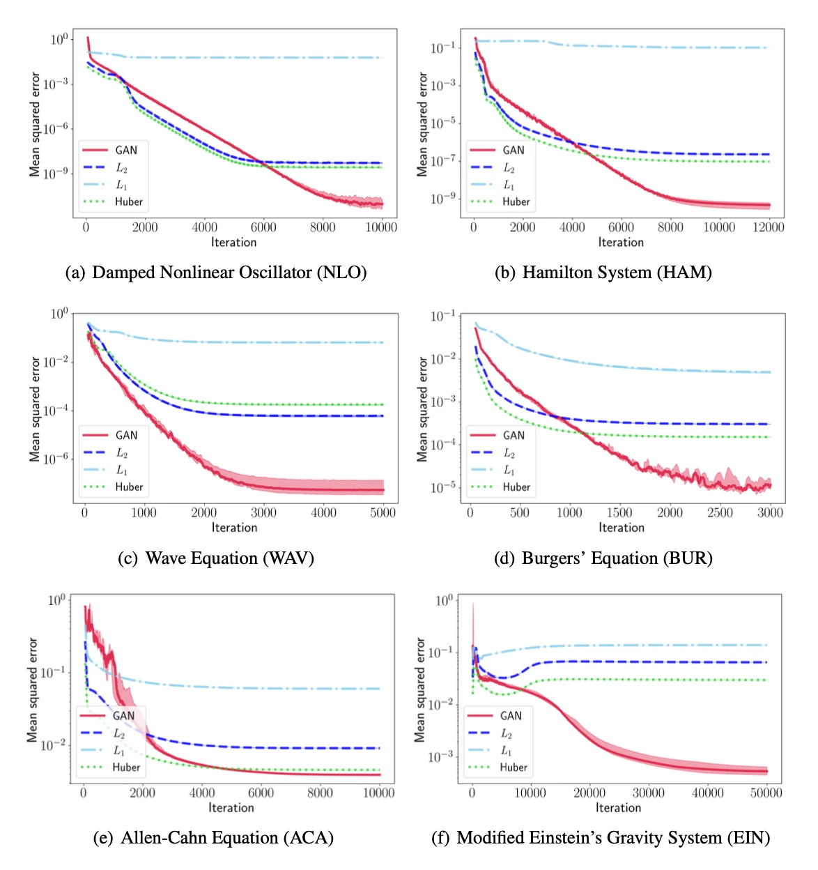
DEQGAN predictions and errors compared with fixed-loss physics-informed networks.